Download area
Download a tutorial
Download Non Equilibrium software package
Modelling Activity
Non Equilibrium thermodynamics for Glassy Polymers
CFD modeling of fluid transport in solid materials
Non Equilibrium thermodynamics for Glassy Polymers
Introduction
Assumptions and conclusions
Solubility calculation
Model parameters
Some results
References
Introduction: fluid sorption in glassy polymers
Glassy polymers are non equilibrium systems which cannot be described
with conventional equilibrium models and they have higher specific volume
than the equilibrium value.
For the gas sorption in glassy polymers, that is relevant in many applications
as in the membrane separation field, an empricial equation is often used
that relates the amount of fluid abosrbed to the gas phase pressure (or
fugacity), the dual-mode model (1)
![]()
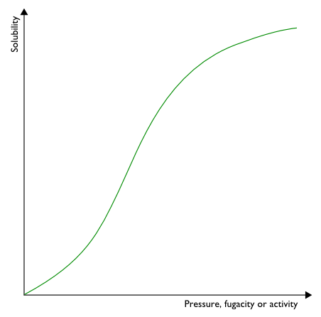
Although this model has been used successfully and extensively over the
years to represent the typical convex shape of solubility isotherms of
glassy polymers, its physical assumptions present an oversimplified picture
of the physico-chemical factors affecting the sorption process. The three
model parameters, kD, C'H
and b, which are obtained by curve-fitting the model to experimental
data, can only be used in the range of temperature and pressure over which
the regression is performed and for the specific penetrant-polymer pair
for which the experimental sorption data were obtained. In this regard,
an extensive study of the dependence of the dual-mode parameters on the
pressure range used for the fitting procedure was presented by Bondar
et al. (2)
These observations imply that this model cannot be used for predictive
purposes. Moreover, the basic physical interpretation of the dual
mode equation cannot be used, even qualitatively, to describe the behavior
of polymer-penetrant pairs, such as alcohols and glassy PTMSP, which exhibit
an S-shaped sorption isotherm. (3)
 Sigmoidal sorption isotherm
(e.g. alcohols in PTMSP)
Sigmoidal sorption isotherm
(e.g. alcohols in PTMSP)
Alternative models have been developed to describe gas solubility in
glassy polymers; these models are generally constructed on a more fundamental
basis than that of the dual mode model. (4-6)
The non-equilibrium lattice fluid (NELF) model, proposed by Doghieri
and Sarti, (7-9) considers a single population of penetrant molecules
dissolved into the glassy polymer. This model can be used in a predictive
way, based only on pure component parameters, and has proven to be
quite satisfactory for all the gas-polymer pairs examined so far. The
glassy state of a polymer is a non-equilibrium phase in which the
Gibbs free energy does not correspond to the minimum attainable value.
The NELF model relies on the hypothesis that the Gibbs free energy of
a glassy polymer can be described by considering the density of the
polymer to be an internal state variable. The NELF model adopts from
the equilibrium Gibbs free energy expression for polymer mixtures proposed
for the lattice fluid theory by Sanchez and Lacombe.(10-11) The
gas solubility is calculated from the phase equilibrium condition, which
requires equality between the chemical potential of the penetrant species
in the glassy polymer and in the external gaseous phase.
The NELF model was then generalized in order to account for more recent
and accurate Equation of State Models giving rise to the so called NET
GP approach (Non Equilibrium thermodynamics for Glassy Polymers) which
is interfaced to Perturbedh Hard Sphere Chain (PHSC) and Statistical Associating
Fluid Theory (SAFT) Equations of State.
The glassy polymeric phase is
i) homogeneous ii) isotropic iii) amorphous
The glassy phase reaches an asymptotic pseudo equilibrium condition
According to these assumptions it can be demonstrated that:
the non-equilibrium Helmholtz free energy,in a general non-equilibrium
state coincides with the corresponding property evaluated on the equilibrium
curve at the same T, p, and composition:
![]()
Similarly, the chemical potential per unit mass of solute i in the glassy
phase is given by:
![]()
Therefore, once an expression for aEQ is selected for the polymer-penetrant
mixture, the corresponding non-equilibrium equation is readily obtained
. Such results are derived in general terms and are independent of the
particular EoS model used for the free energy
Non-equilibrium free energy functions are given by different Equations
of State (EoS) models as :
Lattice Fluid (LF),(10-11)

Statistical Associating Fluid Theory (SAFT) and PC-SAFT,(12-15)
Perturbed Hard Sphere Chain (PHSC) model (16-18 )
and give rise to the corresponding non-equilibrium models indicated as
NELF, NE-SAFT and NE-PHSC, respectively. The non-equilibrium
information is represented by the value of pol, which must be measured
experimentally and cannot be calculated from the equilibrium EoS.
Solubility calculation
In the case of true thermodynamic phase equilibrium, solubility is evaluated
by equating the equilibrium chemical potential of the j-th penetrant in
the polymeric solid to that in the external fluid phase, using also the
equilibrium value of the polymer density given by the equation of state
at that T, p and composition.
![]()
In the pseudo-equilibrium state of a glassy polymer, the relaxation of
polymeric density with time is kinetically hindered; its value becomes
asymptotically constant in time, even though it is not equal to the true
equilibrium value. Under these conditions, the time rate of change of
rho becomes negligibly small, though not exactly equal to zero, while
the equation representing true thermodynamic equilibrium (minimization
of Gibbs free energy)is not obeyed.
The polymer density value during sorption is normally not available at
all penetrant activities and that is a constraint for the application
of the NET-GP approach as a completely predictive tool. In several cases
of practical interest, such as at low activity, or for solutes with very
low solubility, the density of the pure glass provides a very good estimate
of the actual polymer density and the NET-GP approach can be applied in
a predictive way.
When swelling agents or higher gas pressures are used, the NET-GP approach
needs some further consideration. In particular, for the gaseous phases
it can be noticed that, generally, the polymer density during sorption
varies linearly with penetrant pressure:(19)
 |
 |
| Variation of polymer density with pressure during gas sorption in different polycarbonates | NELF model prediction of the corresponding solubility isotherms (20) |
where the swelling coefficient, ksw, represents the effect of gas pressure
on glassy polymer density and is a non-equilibrium parameter, depending
on thermomechanical and sorption history of the sample. The value of the
swelling coefficient, ksw, can be obtained, in principle from a single
experimental solubility datum at high pressure for the system under consideration.
(20)
Model parameters
The pure component parameters for the EoS model chosen are obtained by
fitting the EoS calculations to pure component equilibrium data. For the
penetrant, volumetric and/or vapour pressure values are frequently available
and can be used to that aim. For the polymer, one can use volumetric data
as a function of temperature and pressure above the glass transition temperature,
frequently available in the open literature and in some compilations,
(21) in the common case in which the rubbery phase can be reached before
thermal degradation. An example of such procedure is shown in Figure ,
where volumetric data above and below Tg are given for polycarbonate and
the SAFT model is used to fit the data above Tg, the resulting parameters
for the SAFT model are s: =3.043 Å, M/m=25.00
g/mol, u0/k=371 K. (22) The pure component
parameters can also be predicted using experimental PVT dtaa simulated
with molecular dynamics (MD) simulations.(23)
 |
 |
| Fitting of SAFT EoS parameters on experimental PVT data for polycarbonate (22) | Fitting of PC SAFT EoS parameters on MD simulated PVT data for Kapton (23) |
All mixture models for free energy have also one binary interaction parameter, kij, associated to each couple of chemical species, which can be obtained separately, e.g. from gas-polymer equilibrium data in the rubbery phase, when available. In the absence of any direct experimental information, the first order approximation can be used for kij or, alternatively, it can be treated as adjustable parameter as is often done in the thermodynamic studies of liquid-vapor equilibria. For mixtures formed by components of similar chemical structure, the value of kij is essentially equal to 0.0 (regular solution behavior). .
 |
 |
| Prediction of the solubility of n-C6 in Polystyrene below the glass transition (NELF model) and above the glass transition (LF EoS). (23) | Water vapor and liquid solubility in polycarbonate: experimental data and NELF model (24) |
(1) R. M. Barrer, J. A. Barrie, and J. Slater, J. Polym. Sci., 27, 177
(1958)).
(2) V. I. Bondar, Y. Kamiya, and Y. P. Yampol'skii, J. Polym. Sci.: Part
B : Polym. Phys., 34, 369 (1996)) .
(3) F. Doghieri, D. Biavati, and G. C. Sarti, Ind. Eng. Chem. Res., 35,
2420-2430 (1996)).
(4) T. Oishi and J. M. Prausnitz, Ind. Eng. Chem. Proc., Des. Dev., 17,
333 (1978);
(5) R. M. Conforti, T. A. Barbari, P. Vimalchand, and M. D. Donohue, Macromolecules,
24, 3388-3394 (1991);
(6) R. G. Wissinger and M. E. Paulaitis, Ind. Eng. Chem. Res., 30, 842-851
(1991)).
(7) F. Doghieri and G. C. Sarti, Macromolecules, 29, 7885-7896, (1996);
(8) G. C. Sarti and F. Doghieri, Chem. Eng. Sci., 53, 3435-3447, (1998);
(9) F. Doghieri and G. C. Sarti, J. Membr. Sci., 147, 73-86, (1998)
(10) R. H. Lacombe and I. C. Sanchez, J. Phys. Chem., 80, 2568-2580 (1976);
(11) I. C. Sanchez and R. H. Lacombe, J. Polym. Sci.: Polym. Letts. Ed.,
15, 71-75, (1977).
(12) Huang SH, Radosz M. 1990. Ind. Eng. Chem. Res. 29:2284-94
(13) Chapman WG, Gubbins KE, Jackson G, Radosz M. 1989. SAFT. Fluid Phase
Equilib. 52:31-8
(14) Chapman WG, Gubbins KE, Jackson G, Radosz M. 1990. 29:1709-21
(15) Gross, J.; Sadowski, G. Ind. Eng. Chem. Res. 2001, 40, 1244.
(16) Song Y, Hino T, Lambert SM, Prausnitz JM. 1996. 117:69-76
(17) Hino T, Prausnitz JM. 1997. Fluid Phase Equilib. 138:105-130
(18) Song Y, Lambert SM, Prausnitz JM. 1994. Macromolecules. 27:441-48
(19) Wissinger G, Paulaitis ME. 1987. J. Polym. Sci, Part B: Polym. Phys.
25:2497-510.
(20) Giacinti Baschetti M, Doghieri F, Sarti GC. 2001. Ind. Eng. Chem.
Res. 40:3027-37.
(21) Zoller P, Walsh D. 1995. Standard Pressure-Volume-Temperature Data
for Polymers. Lancaster: Technomic
(22) M.G. De Angelis, G.C. Sarti, Annu Rev Chem Biomolec Eng, 2011, 2,
97 - 120
(23) M. Minelli, M.G. De Angelis, D. Hofmann, Fluid Phase Equilibria 2012,
333, 87 - 96
(24) M.G.
De Angelis, G.C. Sarti, AIChE Journal, 2012, 58, 292-301.